Note
Go to the end to download the full example code.
Accessing parcellation maps
Just like reference templates (covered in Accessing brain reference templates), parcellation maps and region maps are 3D volumes, providing spatial representations for their “semantic counterparts” Parcellation and Region in a particular reference space. Just like reference templates, they are Volume objects, describing a 3D volume in image or mesh format. An important difference to reference templates is that parcellation maps also link (valid names of) brain regions to the voxels or vertices in the volume.
Import the package.
import siibra

# We use `nilearn <https://nilearn.github.io>`_ again for plotting.
from nilearn import plotting
Similar to the parcellations, spaces, and atlases, you can access to preconfigured maps by siibra.maps. Additionally, we can use a pandas.DataFrame to navigate the details of these maps and filter them. For example, fetch all the maps defined on “MNI Colin 27” space.
siibra.maps.dataframe.query('space == "MNI Colin 27"')
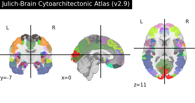
We select the maximum probability map of Julich-Brain in MNI152 space, which is a parcellation map with discrete labels. get_map assumes maptype=’labelled’ by default.
julich_mpm = siibra.get_map(space="icbm 2009c", parcellation="julich 2.9", maptype="labelled")
print(julich_mpm)
Map: mni152 jba29 labelled
Like reference templates, parcellation maps may provide more than one volume to support different formats, especially both mesh and image representations. As already seen for reference templates, to access the actual image data, we call the fetch() method. Per default, this gives us a Nifti1Image object if image data is available for the volume.
assert julich_mpm.provides_image
mapimg = julich_mpm.fetch()
print(type(mapimg))

# we can now plot the image with nilearn. Some maps even provide
# their own predefined colormap for this purpose.
cmap = julich_mpm.get_colormap()
plotting.plot_roi(
    mapimg, title=f"{julich_mpm.parcellation.name}", cmap=cmap
)
<class 'nibabel.nifti1.Nifti1Image'>

<nilearn.plotting.displays._slicers.OrthoSlicer object at 0x7fbc2d04f790>
As we see, this parcellation maps splits the volume into independent fragments, which have been merged when fetching without more specific arguments. We can select a fragment:
mapimg_r = julich_mpm.fetch(fragment='right')
plotting.plot_roi(
    mapimg_r, title=f"{julich_mpm.parcellation.name} (right)", cmap=cmap
)

<nilearn.plotting.displays._slicers.OrthoSlicer object at 0x7fbc2b869640>
Julich-Brain, like some other parcellations, provides probabilistic maps. The maximum probability map is just a simplified representation, displaying for each voxel the label of the brain region with highest probability. We can access the probabilistic information by requesting the “statistical” maptype (siibra.maptype.STATISTICAL). Note that since the set of probability maps are usually a large number of sparsely populated image volumes, siibra will load the volumetric data only once and then convert it to a sparse index format, that is much more efficient to process and store. The sparse index is cached on the local disk, therefore subsequent use of probability maps will be much faster.
julich_pmaps = siibra.get_map(
    space="mni152",
    parcellation="julich 2.9",
    maptype="statistical",
)
julich_pmaps

# Since the statistical maps overlap, this map provides access to several
# hundreds of brain volumes.
print("Number of regions:", len(julich_pmaps))

# We can iterate over all probability maps using `fetch_iter()`.
# Here we just display the first map.
pmap = next(iter(julich_pmaps))
plotting.plot_stat_map(pmap, cmap='viridis')

# Of course, we do not know which region this first volume belongs to,
# but the parcellation map object can decode this for us:
julich_pmaps.get_region(volume=0)

Number of regions: 296

Ch 123 (Basal Forebrain) left
When accessing probabilistic maps, we typically want to fetch the volume corresponding to a particular brain region instead of selecting the volume by iteration order. We can do this by using the index of a region explicitly:
v1l_index = julich_pmaps.get_index('v1 left')
v1l_pmap = julich_pmaps.fetch(index=v1l_index)

# For convenience, we can specify the region name
# in fetch() right away, and let the parcellation map
# translate the index in the background:
v1l_pmap = julich_pmaps.fetch(region="v1 left")
plotting.plot_roi(v1l_pmap, title="v1 left", cmap='viridis')

<nilearn.plotting.displays._slicers.OrthoSlicer object at 0x7fbc2d04f760>
In addition to parcellation maps, siibra can produce binary masks of brain regions.
hoc5L = siibra.get_region(parcellation='julich 2.9', region='hoc5 left')
hoc5L_mask = hoc5L.fetch_regional_map(space="mni152", maptype="labelled")
plotting.plot_roi(hoc5L_mask, title=f"Mask of {hoc5L.name}")

<nilearn.plotting.displays._slicers.OrthoSlicer object at 0x7fbc2b517340>
Total running time of the script: (0 minutes 21.136 seconds)