
Note
Go to the end to download the full example code.
Case study: Anatomical evaluation of subcortical maps
This notebook uses siibra to re-assess some results of the study “Ventral intermediate nucleus structural connectivity-derived segmentation: anatomical reliability and variability”, [Bertino et al., NeuroImage 2021](https://doi.org/10.1016/j.neuroimage.2021.118519).
The study tested different parcellation pipelines for tractography-derived putative Vim identification. Thalamic parcellation was performed on a high quality, multi-shell dataset and a downsampled, clinical-like dataset using two different diffusion signal modeling techniques and two different voxel classification criteria. Of the resulting four parcellation pipelines, the most reliable in terms of inter-subject variability has been picked and parcels putatively corresponding to motor thalamic nuclei have been selected by calculating similarity with a histology-based mask of Vim. The effect of data quality and parcellation pipelines on a volumetric index of connectivity clusters has been assessed.
- For the different non-invasive parcellations, the study investigates
reliability across subjects
anatomical plausibility with respect to the histological mask from Morel/Krauth, NeuroImage 2010
relationship to clinically relevant tremor stimulation targets
- Main findings include:
CSD+THR pipeline is most reliable
Precentral SMA and dentatus coincide most with the histological masks
dentatus-linked thalamus voxels are closest to optimal stimulation points from the literature; however with high variability
volumina of parcels vary significantly per pipeline and data quality, thus target planning should not be done purely from the tractography-parcellation results
import siibra
from nilearn import plotting
import matplotlib.pyplot as plt
import numpy as np
import pandas as pd
from shapely.geometry import MultiPoint
from shapely import concave_hull, geometry, intersection
import re
import requests
import nibabel as nib
from nilearn.image import resample_to_img
1. Identify cluster maps coinciding with VIM
The study computes DICE scores of the extracted thalamic clusters to histology-based atlas masks from the DISTAL atlas, to evaluate overlap with known region delineations. We use the Julich-Brain atlas, wnich provides probabilistic maps of these subregions, to re-assess these overlap scores.
1.1 Load cluster maps
cluster_names = [
    "Precentral",
    "Dentate",
    "SMA",
    "Paracentral",
    "Postcentral",
    "Temporal",
    "Occipital",
    "Parietal",
    "Prefrontal",
]
hemispheres = {"left": "L", "right": "R"}
utility function to load a mask that is resampled to a reference voxel volume
def load_resampled_mask(uri, ref):
    try:
        nim = nib.load(uri)
    except FileNotFoundError:
        response = requests.get(uri)
        with open("temp.nii.gz", "wb") as f:
            f.write(response.content)
        nim = nib.load("temp.nii.gz")
    return resample_to_img(nim, ref, interpolation="nearest", force_resample=True)
retrieve the cluster maps from the original resource
url_scheme = (
    "https://github.com/BrainMappingLab/"
    "Thalamic-Structural-Connectivity-Based-Parcellation-for-non-invasive-Vim-Identification/"
    "raw/refs/heads/main/{}h/{}_{}_CSDTHR_HQ.nii.gz"
)

clustermaps = {}
mni_template = siibra.get_template("mni152").fetch()
for clustername in cluster_names:
    for hemname, hemcode in hemispheres.items():
        url = url_scheme.format(hemcode.lower(), hemcode, clustername)
        nimg = load_resampled_mask(url, mni_template)
        clustermaps[clustername, hemcode] = siibra.volumes.from_nifti(
            nimg, space="mni152", name=f"{clustername} {hemname}"
        )
/actions-runner/_work/siibra-python/siibra-python/examples/tutorials/2025-paper-fig6.py:97: FutureWarning: From release 0.13.0 onwards, this function will, by default, copy the header of the input image to the output. Currently, the header is reset to the default Nifti1Header. To suppress this warning and use the new behavior, set `copy_header=True`.
  return resample_to_img(nim, ref, interpolation="nearest", force_resample=True)
Hemispheres of Dentate cluster maps are confused in the study data
tmp = clustermaps["Dentate", "L"]
clustermaps["Dentate", "L"] = clustermaps["Dentate", "R"]
clustermaps["Dentate", "R"] = tmp
1.2 Reported DICE scores with DISTAL atlas
The paper reports on average DICE scores with each subject in the individual subject spaces. We fill the reported values in a dataframe as a starting point.
Reported average within-subject scores in the paper
cluster_scores = pd.DataFrame(
    [
        ["Precentral", "L", 0.25],
        ["Precentral", "R", 0.30],
        ["Dentate", "L", 0.27],
        ["Dentate", "R", 0.27],
        ["SMA", "L", 0.22],
        ["SMA", "R", 0.20],
        ["Paracentral", "L", 0.18],
        ["Paracentral", "R", 0.20],
        ["Postcentral", "L", 0.08],
        ["Postcentral", "R", 0.11],
        ["Prefrontal", "L", 0.14],
        ["Prefrontal", "R", 0.12],
        ["Parietal", "L", 0.01],
        ["Parietal", "R", 0.00],
        ["Temporal", "L", 0.00],
        ["Temporal", "R", 0.00],
        ["Occipital", "L", 0.00],
        ["Occipital", "R", 0.00],
    ],
    columns=["Cluster name", "Hemisphere", "Dice score (study)"],
)
cluster_scores.set_index(["Cluster name", "Hemisphere"], inplace=True)
cluster_scores
1.3 Assign clustermaps to Julich-Brain via probability maps correlation
Perform probabilistic assignment for each clustermap
julichbrain = siibra.parcellations.get("julich 3.1")
pmaps = julichbrain.get_map(space="mni152", maptype="statistical")
assignments = {}
for (clustername, hemcode), clustermap in clustermaps.items():
    with siibra.QUIET:
        df = pmaps.assign(clustermap, split_components=False)
    df.set_index("region", inplace=True)
    df.sort_values(by="correlation", ascending=False, inplace=True)
    assignments[clustername, hemcode] = df
Extract vim correlations and maximum correlations from the probabilistic assignments and update cluster scores.
vim_regions = {c: julichbrain.get_region(f"vim {n}") for n, c in hemispheres.items()}
vim_correlations = {}  # correlation of each clustermap with Julich-Brain VIM
best_correlations = (
    {}
)  # best correlation of each clustermap with any Julich-Brain regiob
best_regions = (
    {}
)  # Name of Julich-Brain region with best correlation to each clustermap
for (clustername, hemcode), df in assignments.items():
    # collect highest score and corresponding region
    best_regions[clustername, hemcode] = df.iloc[0].name
    best_correlations[clustername, hemcode] = df.iloc[0].loc["correlation"]
    vim = vim_regions[hemcode]
    if vim in df.index:
        vim_correlations[clustername, hemcode] = df.loc[vim].correlation.iloc[0]
    else:
        vim_correlations[clustername, hemcode] = 0

# add results to assignment table
cluster_scores["Julich-Brain Correlation (VIM)"] = vim_correlations
cluster_scores["Julich-Brain Correlation (best)"] = best_correlations
cluster_scores["Julich-Brain region"] = best_regions
cluster_scores.round(2)
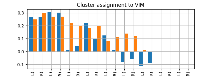
Observations
1. By filtering strong correlations to the VIM probability map in Julich-Brain, we can confirm the cluster selection from the paper. Precentral and Dentate are even more distinct than the DICE scores in the paper. 2. For Precentral, our assignment suggests that the correlation is stronger to the neighboring nucleus VLP rather than the VIM.
Bar plot of Distal dice scores versus Julich-Brain correlations
plt.figure(layout="constrained")
cluster_scores.plot(
    kind="bar",
    y=["Julich-Brain Correlation (VIM)", "Dice score (study)"],
    grid=True,
    figsize=(7, 2.5),
    width=0.8,
    title="Cluster assignment to VIM",
)
plt.legend(
    [
        "Correlation with Julich-Brain probabilistic maps",
        "Dice score with Distal atlas (study)",
    ],
    loc="center left",
    bbox_to_anchor=(0.15, -1.0),
)
<matplotlib.legend.Legend object at 0x7fc19f1a8cd0>
2. Investigate in histology data
We use siibra to retrieve 1-micrometer histology sections in the regions of interest, and to compare the fit of map contours with the actual histology. We show projected contours of 1. the clustermap, 2. the DISTAL VIM map, 3. Julich-Brain probability maps of VIM, and 4. Julich-Brain probability map of the best assigned region.
Define a few utility functions
def points_from_volume(volume: siibra.volumes.Volume, thres: float = 0.):
    # Create a siibra pointcloud of corresponding to nonzero voxels of theresholded volume
    img = volume.fetch()
    arr = img.get_fdata()
    coords = np.argwhere(arr > thres)
    if len(coords) == 0:
        return None
    return siibra.PointCloud(coords, labels=arr[tuple(coords.T)]).transform(
        img.affine, space=volume.space
    )


def coronal_contour(
    pointcloud: siibra.PointCloud, y: float, ratio: float = 0.
) -> siibra.locations.Contour:
    if pointcloud is None:
        return None
    # get the 2D contour of the pointcloud in the given y plane
    hull = concave_hull(
        MultiPoint([[x_, z_] for x_, y_, z_ in pointcloud if abs(y_ - y) <= 1.0]),
        ratio=ratio,
    )
    if len(hull.exterior.coords) == 0:
        return None
    return siibra.locations.Contour(
        [(x, y, z) for x, z in hull.exterior.coords], space=pointcloud.space
    )


bigbrain_contour = lambda vol, y, thres: coronal_contour(
    points_from_volume(
        volume=vol,
        thres=thres
    ).warp("bigbrain"),
    y=y,
    ratio=0.5
)


def get_best_section(volume: siibra.volumes.Volume, thres: float = 0.):
    pts_bb = points_from_volume(volume=volume, thres=thres).warp("bigbrain")
    sections = siibra.features.get(pts_bb.boundingbox, "CellbodyStainedSection")
    point_intersections = [
        pts_bb.intersection(s.get_boundingbox().zoom(2))
        for s in sections
    ]
    best_index = np.argmax([
        0 if pts is None else len(pts)
        for pts in point_intersections
    ])
    best_section = sections[best_index]
    print(f"Best section for {clustername} {hem} is {best_section}")
    return best_section


shortname = lambda n: re.sub(r"\s*\(.*\)", "", n)  # shorten area names for figures
2.1 Load the reference contour in section 3797
d = requests.get(
    "https://raw.githubusercontent.com/FZJ-INM1-BDA/siibra-python/refs/heads/main/examples/tutorials/e2ec8c09.sands.json"
).json()
vim_reference = siibra.PointCloud(
    [[v["value"] for v in c] for c in d["coordinates"]], space="bigbrain"
)
section_spec = "3797"  # set the specification for later use
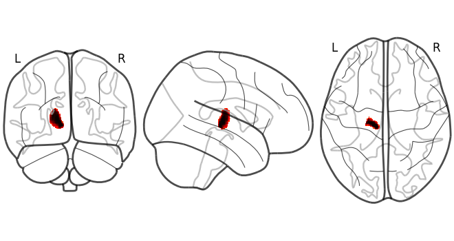
Set a cluster and plot its map and correlation
clustername = "Precentral"
hem = "left"
hemcode = hemispheres[hem]
clustermap = clustermaps[clustername, hemcode]
plotting.plot_glass_brain(clustermap.fetch())
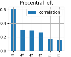
df = assignments[clustername, hemcode].query("correlation > 0.1")[["correlation"]]
df.index = [re.sub(r"\s*\(.*?\)", "", r.name) for r in df.index]
df.plot(kind="bar", figsize=(2.5, 2), grid=True, title=f"{clustername} {hem}")
plt.tight_layout()
2.2 Extract patch from BigBrain
best_section = get_best_section(clustermap)
section = [
    s
    for s in siibra.features.cellular.CellbodyStainedSection._get_instances()
    if section_spec in s.name
][0]
print(f"Section: {section.name[1:5]}")

# Get y-axis in BigBrain of the section's center
y_bigbrain = section.get_boundingbox().center[1]
print("y:", y_bigbrain)
Best section for Precentral left is CellbodyStainedSection #3556: selected 1 micron scans of BigBrain histological sections (v1.0) (cell body staining) in space BigBrain microscopic template (histology)
Section: 3797
y: 5.920500000000001
2.3 Load DISTAL Atlas (Ewert 2017)
DISTAL Atlas can be found at https://www.lead-dbs.org/helpsupport/knowledge-base/atlasesresources/distal-atlas/ UNCOMMENT the lines below if you have a license to use DISTAL Atlas (Ewert 2017).
# distalmap_path = ""
# distalmap = nib.load(distalmap_path)
# vim_map_distal = distalmap[hemcode]
2.4 Plot map contours
vim_map_jba = julichbrain.get_region(f"vim {hem}").get_regional_map("mni152")
best_region_jba = cluster_scores.loc[clustername, hemcode]["Julich-Brain region"]
best_map_jba = best_region_jba.get_regional_map("mni152")
contours = {
    f"Cluster {clustername} {hem}": (
        "k",
        bigbrain_contour(clustermap, y_bigbrain, 0.0),
    ),
    # UNCOMMENT the line below if you have a license to use DISTAL Atlas (Ewert 2017)
    # f"VIM {hem} (Distal)": ("m", bigbrain_contour(vim_map_distal, y_bigbrain, 0.5)),
    f"{shortname(best_region_jba.name)} (Julich-Brain)": (
        "b",
        bigbrain_contour(best_map_jba, y_bigbrain, 0.5),
    ),
    f"VIM {hem} (Julich-Brain)": ("r", bigbrain_contour(vim_map_jba, y_bigbrain, 0.5)),
}
if hem == "left" and section_spec in section.name:
    contours["VIM reference annotation"] = ("g", vim_reference)
2.5 Extract patch
x0, _, z0 = np.array([c.coordinates.min(0) for _, c in contours.values() if c is not None]).min(0) - 1
x1, _, z1 = np.array([c.coordinates.max(0) for _, c in contours.values() if c is not None]).max(0) + 1
y0 = section.get_boundingbox().minpoint[1]
y1 = section.get_boundingbox().maxpoint[1]
voi = siibra.BoundingBox([x0, y0, z0], [x1, y1, z1], space="bigbrain")
patch = section.fetch(voi=voi, resolution_mm=0.02)
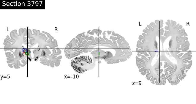
2.6 Display patch with contours
Whole brain view of BigBrain patch
tpl = voi.space.get_template().fetch(resolution_mm=0.8)
view = plotting.plot_img(
    img=patch,
    bg_img=tpl,
    cmap="gray",
    title=f"Section {section.name[1:5]}",
    colorbar=False,
)
for color, cont in contours.values():
    if cont is not None:
        view.add_markers(cont.as_list(), marker_size=0.2, marker_color=color)
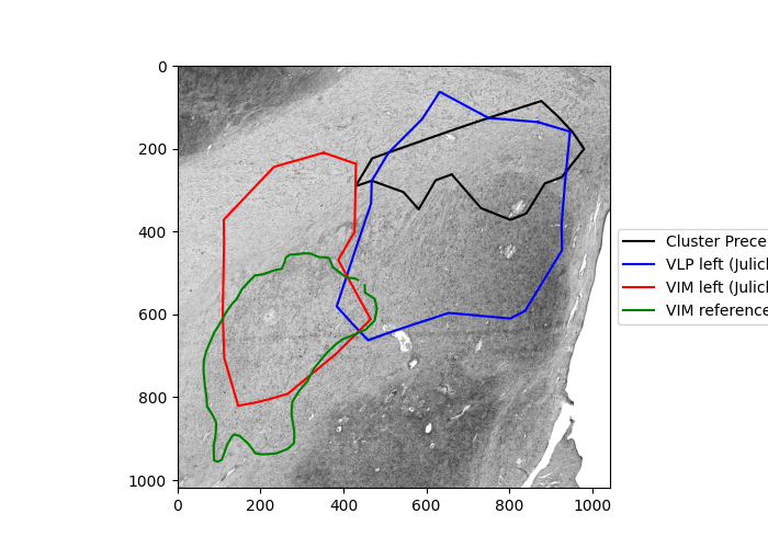
Detailed patch view
plt.figure(figsize=(10, 5))
plt.imshow(patch.get_fdata().squeeze(), cmap="gray")
for name, (color, cont) in contours.items():
    if cont is not None:
        Vx, Vy, Vz = np.dot(np.linalg.inv(patch.affine), cont.homogeneous.T)[:3]
        plt.plot(Vz, Vx, color=color, label=name)
plt.legend(loc="center left", bbox_to_anchor=(1, 0.5))
<matplotlib.legend.Legend object at 0x7fc15a289ad0>
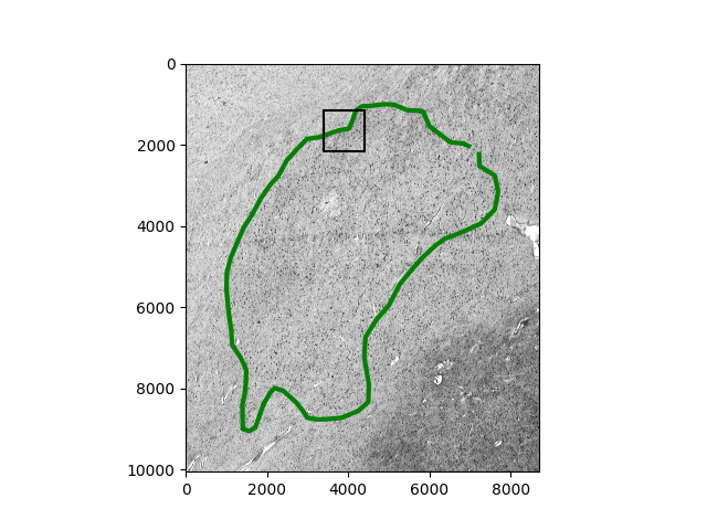
Detailed view of VIM reference alone
# fetch the bounding box
x0, _, z0 = vim_reference.coordinates.min(0) - 1
x1, _, z1 = vim_reference.coordinates.max(0) + 1
ref_voi = siibra.BoundingBox([x0, y0, z0], [x1, y1, z1], space="bigbrain")
ref_patch = section.fetch(voi=ref_voi, resolution_mm=-1)

# plot patch and the reference
plt.figure()
plt.imshow(ref_patch.get_fdata().squeeze(), cmap="gray")
Vx, Vy, Vz = np.dot(np.linalg.inv(ref_patch.affine), vim_reference.homogeneous.T)[:3]
plt.plot(Vz, Vx, color="g", lw=3)

# plot the box of interest
y_, x_ = 1150, 3400
w = 1000
plt.plot([x_, x_, x_ + w, x_ + w, x_], [y_, y_ + w, y_ + w, y_, y_], "k-")

[<matplotlib.lines.Line2D object at 0x7fc159dce2d0>]
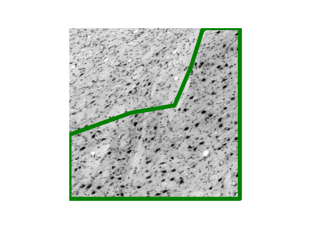
Cellular detail of the patch and VIM reference at the box of interest
plt.figure()
plt.imshow(ref_patch.get_fdata().squeeze()[y_:y_ + w, x_:x_ + w], cmap="gray")
Vx, Vy, Vz = np.dot(np.linalg.inv(ref_patch.affine), vim_reference.homogeneous.T)[:3]
polygon = geometry.Polygon(np.array([Vz - x_, Vx - y_]).T)
canvas = geometry.Polygon([[0, 0], [0, w], [w, w], [w, 0], [0, 0]])
X, Y = intersection(polygon, canvas).exterior.xy
plt.plot(X, Y, color="g", lw=6)
plt.axis("off")
(np.float64(-0.5), np.float64(1050.025), np.float64(1050.025), np.float64(-0.5))
Total running time of the script: (5 minutes 11.273 seconds)
Estimated memory usage: 1937 MB