Note
Go to the end to download the full example code.
Connectivity matrices
siibra provides access to parcellation-averaged connectivity matrices. Several types of connectivity are supported. As of now, these include “StreamlineCounts”, “StreamlineLengths”, and “FunctionalConnectivity”.
from nilearn import plotting
import siibra
We start by selecting an atlas parcellation.
jubrain = siibra.parcellations.get("julich 2.9")
The matrices are queried as expected, using siibra.features.get, passing the parcellation as a concept. Here, we query for structural connectivity matrices.
Found 2 streamline count matrices.
We fetch the first result, which is a specific StreamlineCounts object expressing structural connectivity in the form of numbers of streamlines connecting pairs of brain regions as estimated from tractography on diffusion imaging. Typically, connectivity features provide a range of region-to-region connectivity matrices for different subjects from an imaging cohort.
conn = features[0]
print(f"Connectivity features reflects {conn.modality} of {conn.cohort} cohort.")
print(conn.name)
print("\n" + conn.description)

# Subjects are encoded via anonymized ids:
print(conn.subjects)
Connectivity features reflects StreamlineCounts of HCP cohort.
StreamlineCounts (StreamlineCounts) anchored at minds/core/parcellationatlas/v1.0.0/94c1125b-b87e-45e4-901c-00daee7f2579-290 with cohort HCP

Nowadays, connectivity patterns of brain networks are of special interest, as they may reflect communication in the brain at the structural and functional levels. Their extraction, however, is a complex process that requires deep knowledge of magnetic resonance imaging (MRI) data processing methods. Furthermore, there is no consensus as to which parcellation of the brain is most suitable for a given analysis. Therefore, 19 different state-of-the-art cortical parcellations were used in this dataset to reconstruct the region-based empirical structural connectivity (representing the anatomy of axonal tracts) and functional connectivity (representing the temporal correlation between neuronal activity of brain regions) from diffusion-weighted (dwMRI) and resting-state functional magnetic resonance imaging (fMRI) data, respectively. The repository provides individual connectomes for 200 subjects from the Human Connectome Project. The data can be used by members of the neuroimaging community to investigate structural and functional human connectomes, and to extend the investigation to whole-brain models for further analyses of brain structure and function.
['000', '001', '002', '003', '004', '005', '006', '007', '008', '009', '010', '011', '012', '013', '014', '015', '016', '017', '018', '019', '020', '021', '022', '023', '024', '025', '026', '027', '028', '029', '030', '031', '032', '033', '034', '035', '036', '037', '038', '039', '040', '041', '042', '043', '044', '045', '046', '047', '048', '049', '050', '051', '052', '053', '054', '055', '056', '057', '058', '059', '060', '061', '062', '063', '064', '065', '066', '067', '068', '069', '070', '071', '072', '073', '074', '075', '076', '077', '078', '079', '080', '081', '082', '083', '084', '085', '086', '087', '088', '089', '090', '091', '092', '093', '094', '095', '096', '097', '098', '099', '100', '101', '102', '103', '104', '105', '106', '107', '108', '109', '110', '111', '112', '113', '114', '115', '116', '117', '118', '119', '120', '121', '122', '123', '124', '125', '126', '127', '128', '129', '130', '131', '132', '133', '134', '135', '136', '137', '138', '139', '140', '141', '142', '143', '144', '145', '146', '147', '148', '149', '150', '151', '152', '153', '154', '155', '156', '157', '158', '159', '160', '161', '162', '163', '164', '165', '166', '167', '168', '169', '170', '171', '172', '173', '174', '175', '176', '177', '178', '179', '180', '181', '182', '183', '184', '185', '186', '187', '188', '189', '190', '191', '192', '193', '194', '195', '196', '197', '198', '199']
The connectivity matrices are provided as pandas DataFrames, with region objects as index.
subject = conn.subjects[0]
matrix = conn.get_matrix(subject)
matrix.iloc[0:15, 0:15]  # let us see the first 15x15
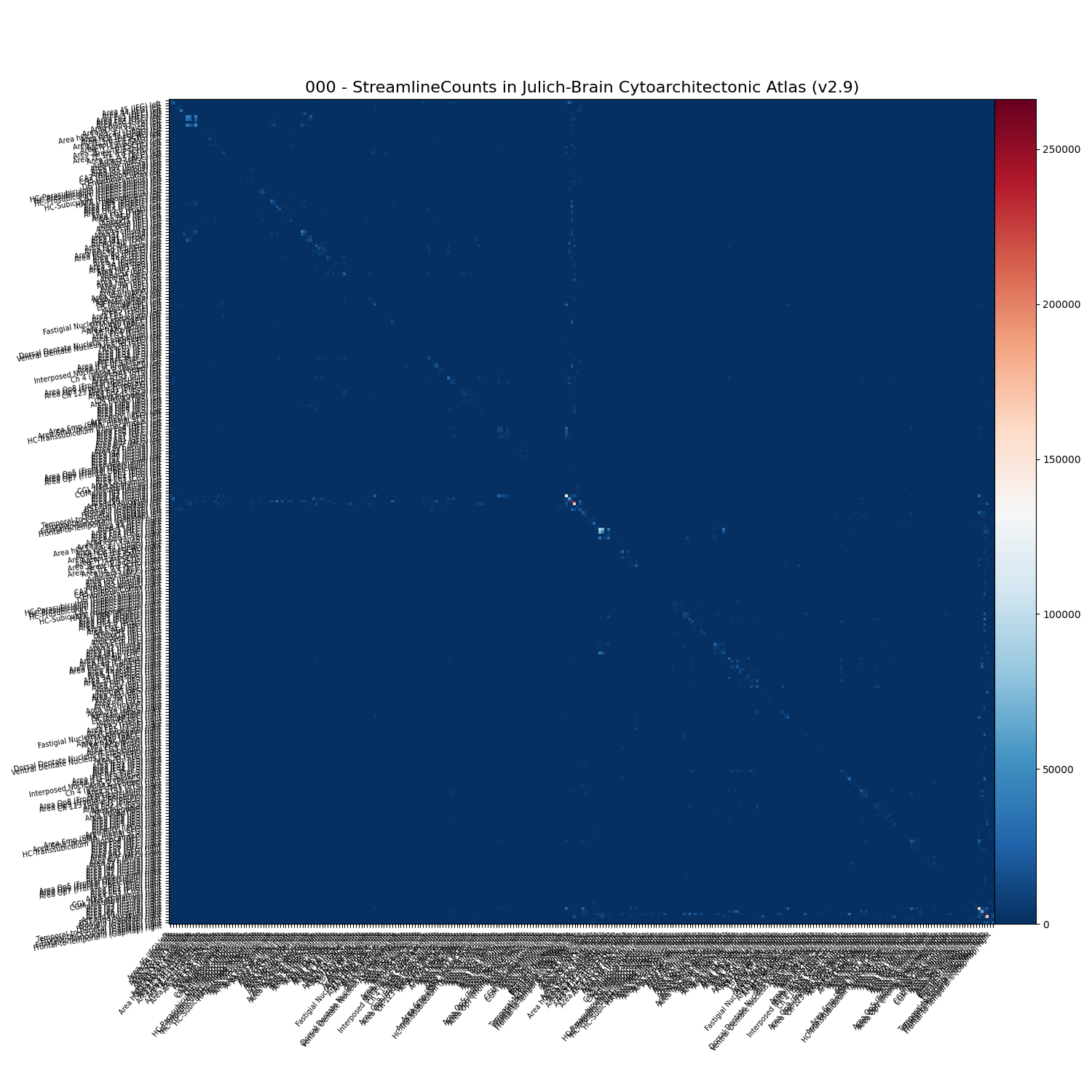
Alternatively, we can visualize the matrix using plot_matrix() method
conn.plot_matrix(subject=conn.subjects[0])
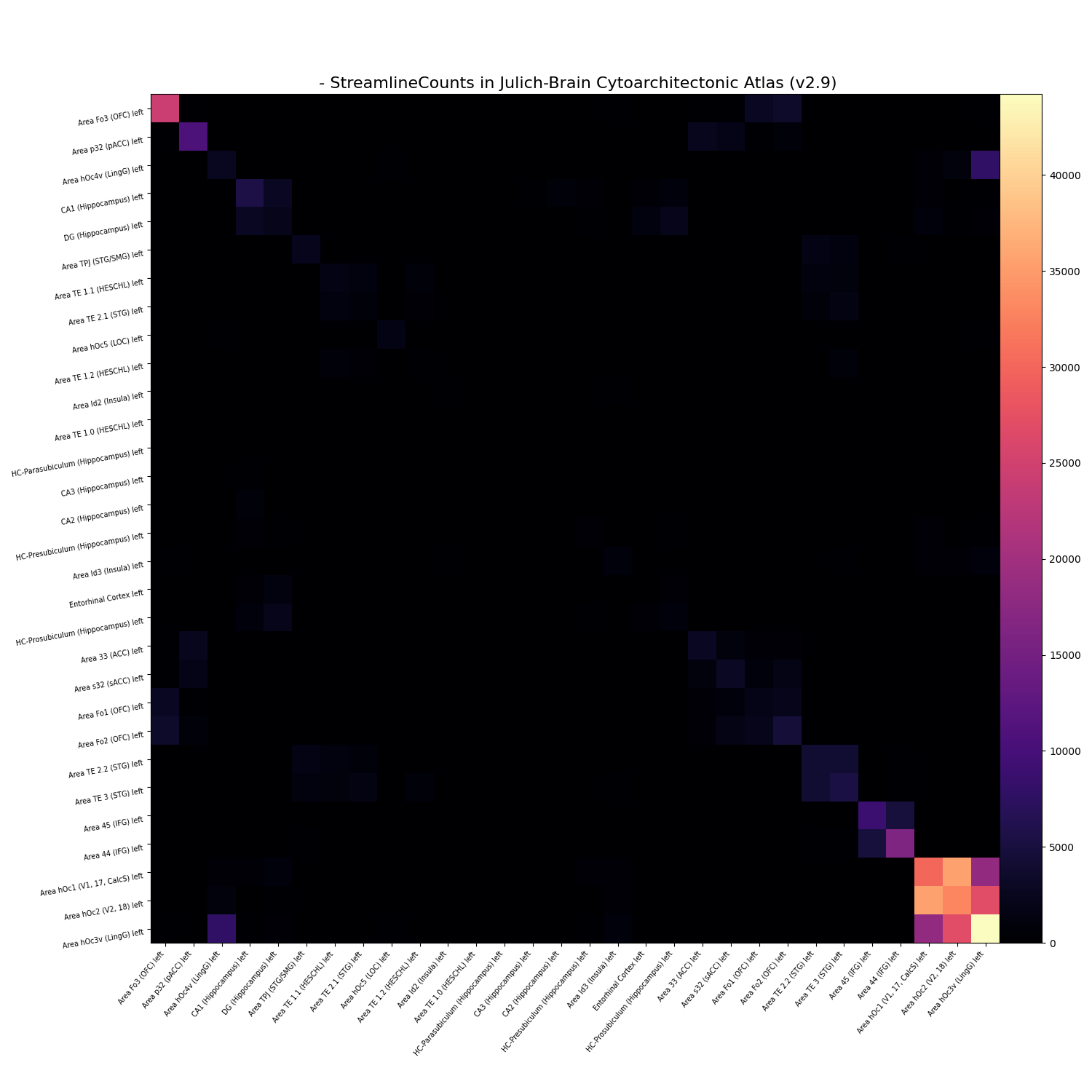
The average matrix across all subjects can be displayed by leaving out subjects or setting it to None. Also, the matrix can be displayed by specifiying a list of regions.
selected_regions = conn.regions[0:30]
conn.plot_matrix(regions=selected_regions, reorder=True, cmap="magma")
We can create a 3D visualization of the connectivity using the plotting module of nilearn. To do so, we need to provide centroids in the anatomical space for each region (or “node”) of the connectivity matrix.
node_coords = conn.compute_centroids('mni152')
/opt/hostedtoolcache/Python/3.8.18/x64/lib/python3.8/site-packages/numpy/core/fromnumeric.py:3464: RuntimeWarning: Mean of empty slice.
  return _methods._mean(a, axis=axis, dtype=dtype,
/opt/hostedtoolcache/Python/3.8.18/x64/lib/python3.8/site-packages/numpy/core/_methods.py:184: RuntimeWarning: invalid value encountered in divide
  ret = um.true_divide(
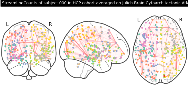
Now we can plot the structural connectome.
view = plotting.plot_connectome(
    adjacency_matrix=matrix,
    node_coords=node_coords,
    edge_threshold="80%",
    node_size=10,
)
view.title(
    f"{conn.modality} of subject {subject} in {conn.cohort} cohort "
    f"averaged on {jubrain.name}",
    size=10,
)
or in 3D:
plotting.view_connectome(
    adjacency_matrix=matrix,
    node_coords=node_coords,
    edge_threshold="99%",
    node_size=3, colorbar=False,
    edge_cmap="bwr"
)
Total running time of the script: (1 minutes 27.962 seconds)