Parcellation-based functional data

siibra provides access to parcellation-averaged functional data such as blood-oxygen-level-dependent (BOLD) signals.

import siibra

We start by selecting an atlas parcellation.

jubrain = siibra.parcellations.get("julich 2.9")

The matrices are queried as expected, using siibra.features.get, passing the parcellation as a concept. Here, we query for structural connectivity matrices.

features = siibra.features.get(jubrain, siibra.features.functional.RegionalBOLD)
print(f"Found {len(features)} parcellation-based BOLD signals for {jubrain}.")

Found 4 parcellation-based BOLD signals for Julich-Brain Cytoarchitectonic Atlas (v2.9).

We fetch the first result, which is a specific RegionalBOLD object.

bold = features[0]
print(f"RegionalBOLD features reflects {bold.modality} of {bold.cohort} cohort.")
print(bold.name)
print("\n" + bold.description)

# Subjects are encoded via anonymized ids:
print(bold.subjects)

RegionalBOLD features reflects Regional BOLD signal of HCP cohort.
RegionalBOLD (Regional BOLD signal) anchored at minds/core/parcellationatlas/v1.0.0/94c1125b-b87e-45e4-901c-00daee7f2579-290 with paradigm rfMRI_REST1_LR_BOLD

Resting-state functional connectivity (FC) is frequently used to predict behavioral, clinical and demographic subject traits. This type of brain connectome can be derived from blood-oxygen-level-dependent (BOLD) signals that reflect the activation of individual brain regions parcellated according to a given brain atlas. Deriving FC from BOLD signals typically involves the estimation of the amount of synchronized coactivations between the BOLD time series of different brain regions. However, several measures of synchronization exist and which one of these metrics is suited best may deviate from study to study. In parallel, the appropriate selection of the brain parcellation is nowadays also still an open issue. This dataset hence comprises the region-based BOLD signals extracted from the resting-state functional magnetic resonance imaging (fMRI) data of 200 healthy subjects included in the Human Connectome Project. The time series were extracted for 20 different state-of-the-art parcellations. The neuroimaging community may use the data of this repository to study, for example, how different measures of synchronization affect the resting-state FC under various parcellation conditions.
['000', '001', '002', '003', '004', '005', '006', '007', '008', '009', '010', '011', '012', '013', '014', '015', '016', '017', '018', '019', '020', '021', '022', '023', '024', '025', '026', '027', '028', '029', '030', '031', '032', '033', '034', '035', '036', '037', '038', '039', '040', '041', '042', '043', '044', '045', '046', '047', '048', '049', '050', '051', '052', '053', '054', '055', '056', '057', '058', '059', '060', '061', '062', '063', '064', '065', '066', '067', '068', '069', '070', '071', '072', '073', '074', '075', '076', '077', '078', '079', '080', '081', '082', '083', '084', '085', '086', '087', '088', '089', '090', '091', '092', '093', '094', '095', '096', '097', '098', '099', '100', '101', '102', '103', '104', '105', '106', '107', '108', '109', '110', '111', '112', '113', '114', '115', '116', '117', '118', '119', '120', '121', '122', '123', '124', '125', '126', '127', '128', '129', '130', '131', '132', '133', '134', '135', '136', '137', '138', '139', '140', '141', '142', '143', '144', '145', '146', '147', '148', '149', '150', '151', '152', '153', '154', '155', '156', '157', '158', '159', '160', '161', '162', '163', '164', '165', '166', '167', '168', '169', '170', '171', '172', '173', '174', '175', '176', '177', '178', '179', '180', '181', '182', '183', '184', '185', '186', '187', '188', '189', '190', '191', '192', '193', '194', '195', '196', '197', '198', '199']

The parcellation-based functional data are provided as pandas DataFrames with region objects as columns and indices as time step.

subject = bold.subjects[0]
table = bold.get_table(subject)
print(f"Timestep: {bold.timestep}")
table[jubrain.get_region("hOc3v left")]

Timestep: 720 ms

0       7218.786845
1       7186.080235
2       7196.478754
3       7162.358546
4       7173.673591
           ...
1195    7206.168284
1196    7210.908622
1197    7187.603819
1198    7204.503983
1199    7203.507897
Name: Area hOc3v (LingG) left, Length: 1200, dtype: float64

We can visualize the signal strength per region by time via a carpet plot. In fact, plot_carpet method can take a list of regions to display the data for selected regions only.

selected_regions = [
    'SF (Amygdala) left', 'SF (Amygdala) right', 'Area Ph2 (PhG) left',
    'Area Ph2 (PhG) right', 'Area Fo4 (OFC) left', 'Area Fo4 (OFC) right',
    'Area 7A (SPL) left', 'Area 7A (SPL) right', 'CA1 (Hippocampus) left',
    'CA1 (Hippocampus) right', 'CA1 (Hippocampus) left', 'CA1 (Hippocampus) right'
]
bold.plot_carpet(subject=bold.subjects[0], regions=selected_regions)

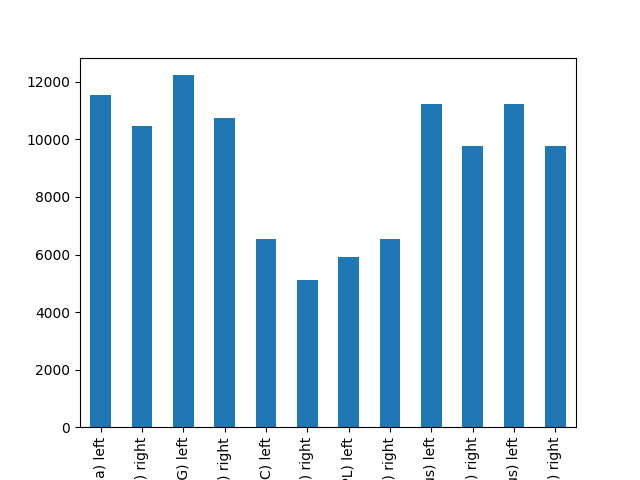
Alternatively, we can visualize the mean signal strength per region:

bold.plot(subject=bold.subjects[0], regions=selected_regions)

<Axes: >