Assigning coordinates to brain regions

siibra can use statistical parcellations maps to make a probabilistic assignment of exact and imprecise coordinates to brain regions. We start by selecting the Julich-Brain probabilistic maps from the human atlas, which we will use for the assignment.

import siibra
from nilearn import plotting

Choose a parcellation map. We demonstrate the use of probabilistic maps here.

with siibra.QUIET:  # suppress progress output
    julich_pmaps = siibra.get_map(
        parcellation="julich 2.9",
        space="mni152",
        maptype="statistical"
    )

Assigning exact coordinate specifications. We now determine the probability values of cytoarchitectonic regions at a an arbitrary point in MNI reference space. The example point is manually chosen. It should be located in PostCG of the right hemisphere. For more information about the siibra.Point class see Locations in reference spaces. The output is a pandas dataframe, which includes the values of different probability maps at the given location. We can sort the table by these values, to see that the region with highest probability is indeed the expected region.

point = siibra.Point((27.75, -32.0, 63.725), space='mni152')
with siibra.QUIET:  # suppress progress output
    assignments = julich_pmaps.assign(point)
assignments.sort_values(by=['map value'], ascending=False)

	input structure	centroid	volume	region	map value
0	0	(27.75, -32.0, 63.72)	43	Area 3b (PostCG) right	0.637676
1	0	(27.75, -32.0, 63.72)	45	Area 1 (PostCG) right	0.179313
2	0	(27.75, -32.0, 63.72)	47	Area 2 (PostCS) right	0.155093
4	0	(27.75, -32.0, 63.72)	247	Frontal-II (GapMap) right	0.105148
3	0	(27.75, -32.0, 63.72)	137	Area 4p (PreCG) right	0.027919

Assigning coordinate specifications with location uncertainty. Typically, coordinate specifications are not exact. For example, we obtain a position from an sEEG electrode, which has several millimeters of uncertainty (especially after warping it to standard space!). If we specify the position with a location uncertainty, siibra will not just read out the values of the probability maps, but instead generate a 3D Gaussian blob with a corresponding standard deviation, and correlate the 3D blob with the maps. We then obtain the weighted average of the map values over the blob, but also additional measures of comparison: A correlation coefficient, the intersection over union (IoU), a containedness score of the blob wrt. the region (“contained”), and a containness score of the region wrt. the blob (“contains”). Per default, the resulting table is sorted by correlation coefficient. Here, we query the assignments with a containedness score of at least 0.5, that is, the regions in which the uncertain point is likely contained.

point_uncertain = siibra.Point((27.75, -32.0, 63.725), space='mni152', sigma_mm=3.)
with siibra.QUIET:  # suppress progress output
    assignments = julich_pmaps.assign(point_uncertain)
assignments.query('`input containedness` >= 0.5').dropna(axis=1)

	input structure	centroid	volume	region	correlation	intersection over union	map value	map weighted mean	map containedness	input weighted mean	input containedness
5	0	(27.75, -32.0, 63.725)	43	Area 3b (PostCG) right	0.223687	0.129916	0.821833	0.375999	0.137754	0.000046	0.695437
6	0	(27.75, -32.0, 63.725)	45	Area 1 (PostCG) right	0.119203	0.143715	0.942186	0.163789	0.160212	0.000034	0.582592
7	0	(27.75, -32.0, 63.725)	47	Area 2 (PostCS) right	0.139431	0.146794	0.797701	0.188924	0.162755	0.000039	0.599504

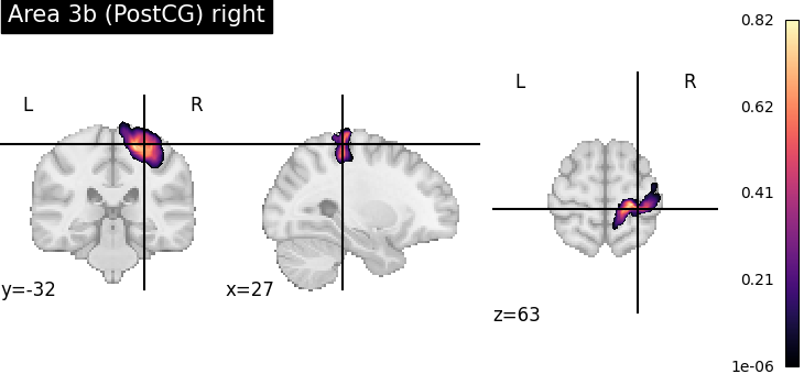
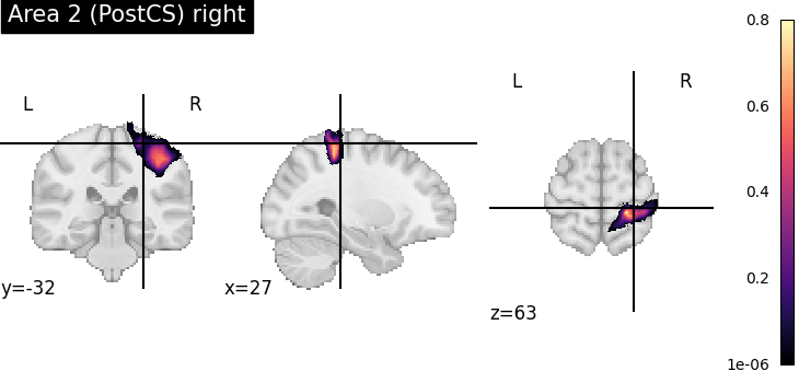
To verify the result, we plot the assigned probability maps at the requested position.

for index, assignment in assignments[assignments['input containedness'] >= 0.5].iterrows():
    pmap = julich_pmaps.fetch(region=assignment['region'])
    plotting.plot_stat_map(pmap, cut_coords=tuple(point), title=assignment['region'], cmap='magma')

• 
• 
•