Neurotransmitter receptor densities

EBRAINS provides transmitter receptor density measurements linked to a selection of cytoarchitectonic brain regions in the human brain (Palomero-Gallagher, Amunts, Zilles et al.). These can be accessed by calling the siibra.features.get() method with feature types in siibra.features.molecular modality, and by specifying a cytoarchitectonic region. Receptor densities come as cortical profiles and regional fingerprints, both tabular style data features.

import siibra

If we query this modality for the whole atlas instead of a particular brain region, all linked receptor density features will be returned.

parcellation = siibra.parcellations.get('julich 2.9')
all_features = siibra.features.get(parcellation, siibra.features.molecular.ReceptorDensityFingerprint)
print("Receptor density fingerprints found at the following anatomical anchors:")
print("\n".join(str(f.anchor) for f in all_features))

Receptor density fingerprints found at the following anatomical anchors:
CA1 (Hippocampus)
CA2 (Hippocampus)
CA3 (Hippocampus)
Area 44 (IFG)
CA2 (Hippocampus)
Area TE 2.1 (STG)
CA1 (Hippocampus)
CA2 (Hippocampus)
CA3 (Hippocampus)
CA1 (Hippocampus)
CA2 (Hippocampus)
CA3 (Hippocampus)
Area PGp (IPL)
CA3 (Hippocampus)
Area PFt (IPL)
CA2 (Hippocampus)
Area 45 (IFG)
Area FG1 (FusG)
CA1 (Hippocampus)
CA2 (Hippocampus)
CA3 (Hippocampus)
Area PFcm (IPL)
Area TE 1.0 (HESCHL)
CA3 (Hippocampus)
Area hOc2 (V2, 18)
CA1 (Hippocampus)
Area 7A (SPL)
Area 3b (PostCG)
Area hOc2 (V2, 18)
Area PF (IPL)
Area FG2 (FusG)
Area PGa (IPL)
Area 4p (PreCG)
CA1 (Hippocampus)
Area hOc3d (Cuneus)
Area 44 (IFG)
Area hOc3v (LingG)
Area PFm (IPL)
Area PFop (IPL)
DG (Hippocampus)
Area hOc1 (V1, 17, CalcS)
DG (Hippocampus)

When providing a particular region instead, the returned list is filtered accordingly. So we can directly retrieve densities for the primary visual cortex:

v1_fingerprints = siibra.features.get(
    siibra.get_region('julich 2.9', 'v1'),
    siibra.features.molecular.ReceptorDensityFingerprint
)
v1_fingerprints[0].plot()

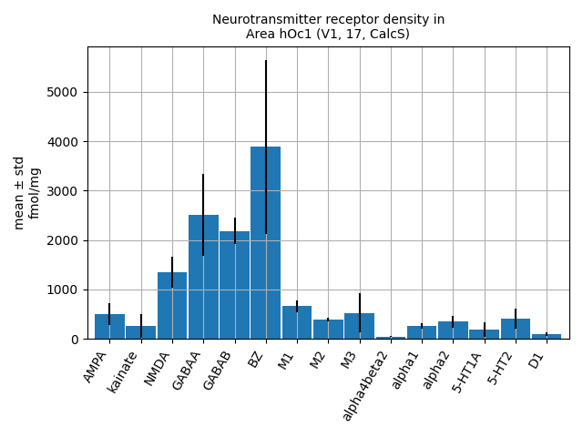
<Axes: title={'center': 'Neurotransmitter receptor density in\nArea hOc1 (V1, 17, CalcS)'}, ylabel='mean ± std\nfmol/mg'>

Each feature includes a data structure for the fingerprint, with mean and standard values for different receptors. The following table thus gives us the same values as shown in the polar plot above:

v1_fingerprints[0].data

	mean	std
receptor
AMPA	500	223
kainate	260	239
NMDA	1348	320
GABAA	2508	828
GABAB	2187	274
BZ	3882	1761
M1	661	123
M2	390	35
M3	524	395
alpha4beta2	48	14
alpha1	264	59
alpha2	347	120
5-HT1A	192	145
5-HT2	408	198
D1	102	37

Many of the receptor features also provide a profile of density measurements at different cortical depths, resolving the change of distribution from the white matter towards the pial surface. The profile is stored as a dictionary of density measures from 0 to 100% cortical depth.

v1_profiles = siibra.features.get(
    siibra.get_region('julich 2.9', 'v1'),
    siibra.features.molecular.ReceptorDensityProfile
)[0]
for p in v1_profiles:
    print(p.receptor)
    if "GABAA" in p.receptor:
        print(p.receptor)
        break
print(p.data)
p.plot()

5-HT1A
5-HT2
alpha1
alpha2
alpha4beta2
AMPA
BZ
D1
GABAA
GABAA
      Receptor density (fmol/mg)
0.00                        1053
0.01                        1101
0.02                        1153
0.03                        1213
0.04                        1274
...                          ...
0.96                         634
0.97                         602
0.98                         580
0.99                         559
1.00                         529

[101 rows x 1 columns]

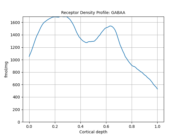
<Axes: title={'center': 'Receptor Density Profile: GABAA'}, xlabel='Cortical depth', ylabel='fmol/mg'>