
Note
Go to the end to download the full example code.
Connectivity matrices
siibra provides access to parcellation-averaged connectivity matrices. Several types of connectivity are supported. As of now, these include “StreamlineCounts”, “StreamlineLengths”, “FunctionalConnectivity”, and “AnatomoFunctionalConnectivity” (F-Tract).
from nilearn import plotting
import siibra
We start by selecting an atlas parcellation.
julich_brain = siibra.parcellations.get("julich 2.9")
The matrices are queried as expected, using siibra.features.get, passing the parcellation as a concept. Here, we query for structural connectivity matrices. Since a single query may yield hundreds of connectivity matrices for different subjects of a cohort, siibra groups them as elements into Compound features. Let us select “HCP” cohort.
features = siibra.features.get(julich_brain, siibra.features.connectivity.StreamlineCounts)
for f in features:
    print(f.name)
    if f.cohort == "HCP":
        cf = f
        print(f"Selected: {cf.name}'\n'" + cf.description)
200 Streamline Counts features cohort: HCP
Selected: 200 Streamline Counts features cohort: HCP'
'Nowadays, connectivity patterns of brain networks are of special interest, as they may reflect communication in the brain at the structural and functional levels. Their extraction, however, is a complex process that requires deep knowledge of magnetic resonance imaging (MRI) data processing methods. Furthermore, there is no consensus as to which parcellation of the brain is most suitable for a given analysis. Therefore, 19 different state-of-the-art cortical parcellations were used in this dataset to reconstruct the region-based empirical structural connectivity (representing the anatomy of axonal tracts) and functional connectivity (representing the temporal correlation between neuronal activity of brain regions) from diffusion-weighted (dwMRI) and resting-state functional magnetic resonance imaging (fMRI) data, respectively. The repository provides individual connectomes for 200 subjects from the Human Connectome Project. The data can be used by members of the neuroimaging community to investigate structural and functional human connectomes, and to extend the investigation to whole-brain models for further analyses of brain structure and function.
349 Streamline Counts features cohort: 1000BRAINS
We can select a specific element by integer index
print(cf[0].name)
print(cf[0].subject)  # Subjects are encoded via anonymized ids
000 - Streamline Counts cohort: HCP
000
The connectivity matrices are provided as pandas DataFrames, with region objects as indices and columns. We can access the matrix corresponding to the selected index by
matrix = cf[0].data
matrix.iloc[0:15, 0:15]  # let us see the first 15x15
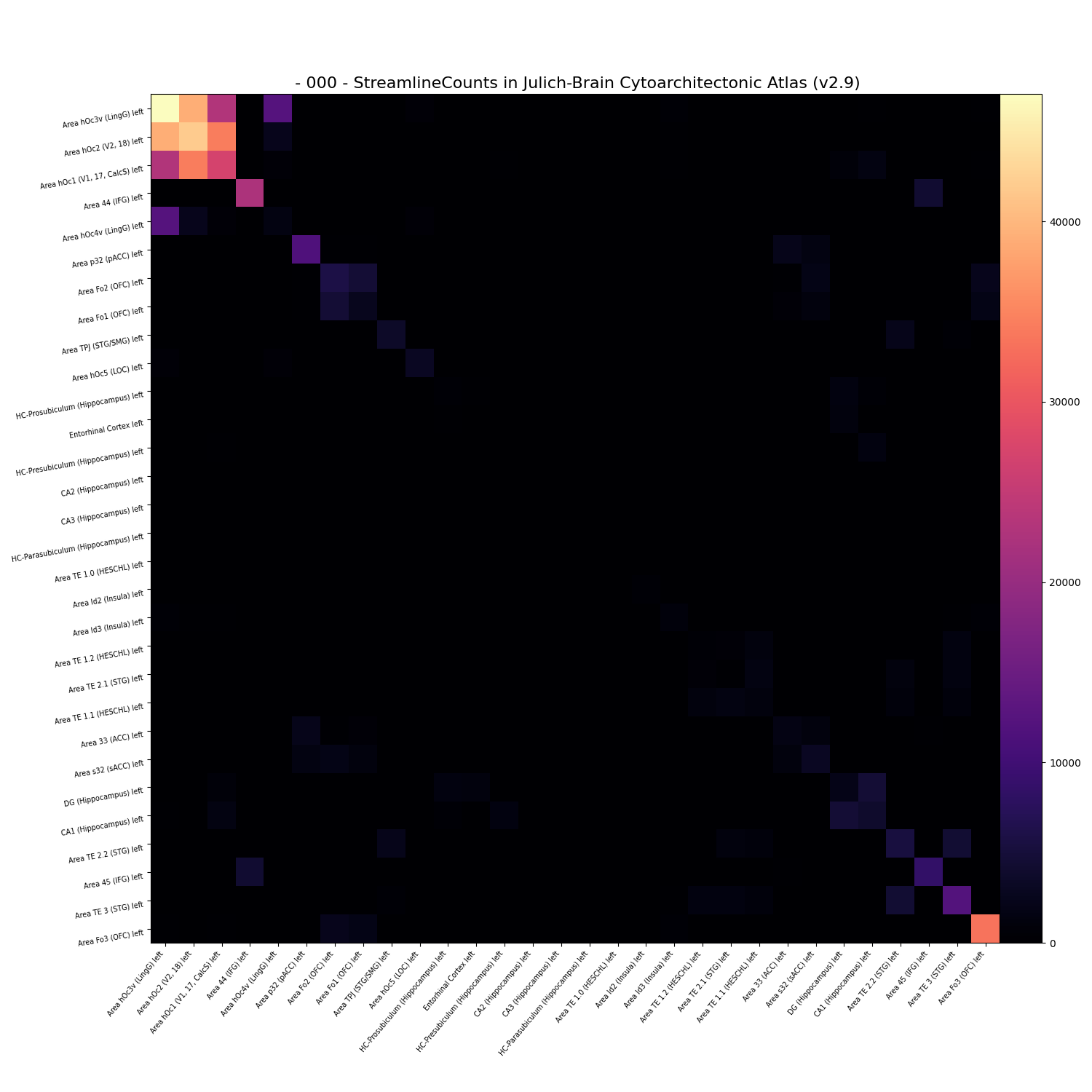
The matrix can be displayed using plot method. In addition, it can be displayed only for a specific list of regions.
selected_regions = cf[0].regions[0:30]
cf[0].plot(regions=selected_regions, reorder=True, cmap="magma")
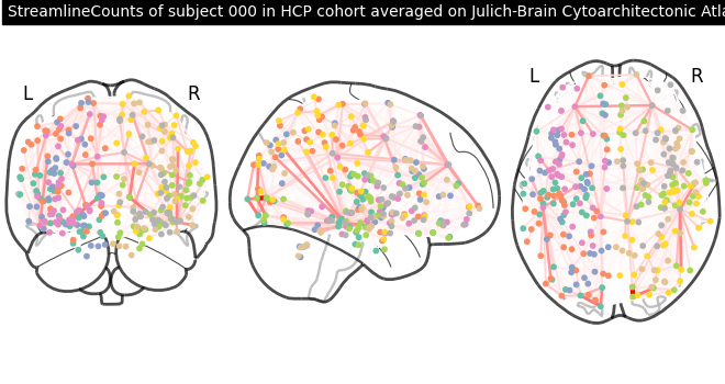
We can create a 3D visualization of the connectivity using the plotting module of nilearn. To do so, we need to provide centroids in the anatomical space for each region (or “node”) of the connectivity matrix.
node_coords = cf[0].compute_centroids('mni152')
Now we can plot the structural connectome.
view = plotting.plot_connectome(
    adjacency_matrix=matrix,
    node_coords=node_coords,
    edge_threshold="80%",
    node_size=10,
)
view.title(
    f"{cf.modality} of subject {cf.indices[0]} in {cf[0].cohort} cohort "
    f"averaged on {julich_brain.name}",
    size=10,
)
or in 3D:
plotting.view_connectome(
    adjacency_matrix=matrix,
    node_coords=node_coords,
    edge_threshold="99%",
    node_size=3, colorbar=False,
    edge_cmap="bwr"
)
You can also access to F-Tract atlases using siibra. Unlike the most connectivity matrices in siibra, F-Tract matrices are subject-averaged but distinguished by their “feature”.
ftract = siibra.features.get(
    siibra.parcellations.get("julich 3.0"),
    siibra.features.connectivity.AnatomoFunctionalConnectivity
)[0]  # also compounded
print(ftract.cohort)
print(ftract.name)
print("indexing attributes:", ftract.indexing_attributes)
for f in ftract:
    print(f.feature)
ADULT PHARMACO-RESISTANT FOCAL EPILEPSY PATIENTS
78 Anatomo Functional Connectivity features cohort: ADULT PHARMACO-RESISTANT FOCAL EPILEPSY PATIENTS
indexing attributes: ('feature',)
P_01: amplitude__mad
P_01: amplitude__median
P_01: dcm_axonal_delay__mad
P_01: dcm_axonal_delay__median
P_01: dcm_excitatory_tc__mad
P_01: dcm_excitatory_tc__median
P_01: dcm_inhibitory_tc__mad
P_01: dcm_inhibitory_tc__median
P_01: duration__mad
P_01: duration__median
P_01: integral__mad
P_01: integral__median
P_01: latency_start__mad
P_01: latency_start__median
P_01: N_implantations
P_01: N_stimulations
P_01: onset_delay__mad
P_01: onset_delay__median
P_01: peak_delay__mad
P_01: peak_delay__median
P_01: probability
P_01: slope__mad
P_01: slope__median
P_01: speed__euclidian__dcm_axonal_delay__mad
P_01: speed__euclidian__dcm_axonal_delay__median
P_01: speed__euclidian__latency_start__mad
P_01: speed__euclidian__latency_start__median
P_01: speed__euclidian__onset_delay__mad
P_01: speed__euclidian__onset_delay__median
P_01: speed__fibres__dcm_axonal_delay__mad
P_01: speed__fibres__dcm_axonal_delay__median
P_01: speed__euclidian__peak_delay__mad
P_01: speed__euclidian__peak_delay__median
P_01: speed__fibres__latency_start__mad
P_01: speed__fibres__latency_start__median
P_01: speed__fibres__onset_delay__mad
P_01: speed__fibres__onset_delay__median
P_01: speed__fibres__peak_delay__mad
P_01: speed__fibres__peak_delay__median
P_11: amplitude__mad
P_11: amplitude__median
P_11: dcm_axonal_delay__mad
P_11: dcm_axonal_delay__median
P_11: dcm_excitatory_tc__mad
P_11: dcm_excitatory_tc__median
P_11: dcm_inhibitory_tc__mad
P_11: dcm_inhibitory_tc__median
P_11: duration__mad
P_11: duration__median
P_11: integral__mad
P_11: integral__median
P_11: latency_start__mad
P_11: latency_start__median
P_11: N_implantations
P_11: N_stimulations
P_11: onset_delay__mad
P_11: onset_delay__median
P_11: peak_delay__mad
P_11: peak_delay__median
P_11: probability
P_11: slope__mad
P_11: slope__median
P_11: speed__euclidian__dcm_axonal_delay__mad
P_11: speed__euclidian__dcm_axonal_delay__median
P_11: speed__euclidian__latency_start__mad
P_11: speed__euclidian__latency_start__median
P_11: speed__euclidian__onset_delay__mad
P_11: speed__euclidian__onset_delay__median
P_11: speed__fibres__dcm_axonal_delay__mad
P_11: speed__fibres__dcm_axonal_delay__median
P_11: speed__euclidian__peak_delay__mad
P_11: speed__euclidian__peak_delay__median
P_11: speed__fibres__latency_start__mad
P_11: speed__fibres__latency_start__median
P_11: speed__fibres__onset_delay__mad
P_11: speed__fibres__onset_delay__median
P_11: speed__fibres__peak_delay__mad
P_11: speed__fibres__peak_delay__median
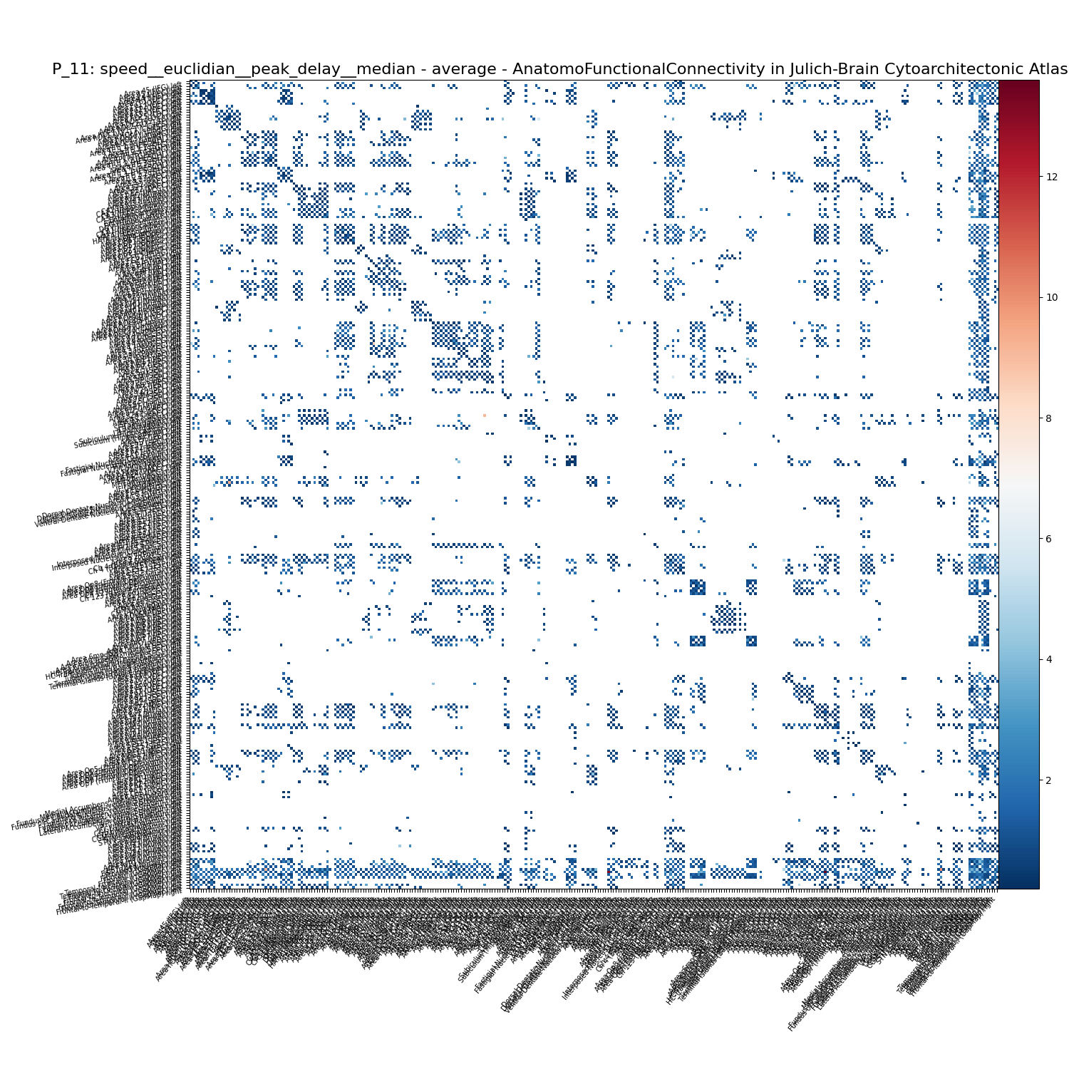
We can similarly draw the data as above. This time let us get the element by its feature name
f = ftract.get_element("P_11: speed__euclidian__peak_delay__median")
f.plot()
Total running time of the script: (4 minutes 31.959 seconds)
Estimated memory usage: 340 MB