Compound features

Some features such as connectivity matrices have attributes siibra can use to combine them into one set, call CompoundFeatures. They allow easy handling of similar features.

Query mechanism for CompoundFeatures is the same as any other. Only difference is that the resulting Feature object has a few extra functionality. Let us demonstrate it with connectivity matrices. They also inherit joint attributes (with the same value) from their elements. Using these, we can distinguish different CompoundFeatures of the same feature type.

import siibra
features = siibra.features.get(siibra.parcellations["julich 2.9"], "StreamlineLengths")
for f in features:
    print("Compounded feature type:", f.feature_type)
    print(f.name)
    if f.cohort == "1000BRAINS":
        cf = f
        print(f"Selected: {cf.name}")

Compounded feature type: <class 'siibra.features.connectivity.streamline_lengths.StreamlineLengths'>
200 Streamline Lengths features cohort: HCP
Compounded feature type: <class 'siibra.features.connectivity.streamline_lengths.StreamlineLengths'>
349 Streamline Lengths features cohort: 1000BRAINS
Selected: 349 Streamline Lengths features cohort: 1000BRAINS

Each of these CompoundFeatures have StreamlineLengths features as elements. We can access to these elements via an integer index or by their key unique to a CompoundFeature using get_element.

print(cf[5].name)
print(cf.get_element('0031_2').name)

0031_2 - Streamline Lengths cohort: 1000BRAINS
0031_2 - Streamline Lengths cohort: 1000BRAINS

The element key changes based on the type of features that make up a CompoundFeature. CompoundFeatures composed of StreamlineLengths obtain their element key from the subject id.

for i, f in enumerate(cf[:10]):  # we can iterate over elements of a CompoundFeature
    print(f"Element index: {cf.indices[i]}, Subject: {f.subject}")

Element index: 0056_1, Subject: 0056_1
Element index: 0152_1, Subject: 0152_1
Element index: 0162_1, Subject: 0162_1
Element index: 0027_1, Subject: 0027_1
Element index: 0142_1, Subject: 0142_1
Element index: 0031_2, Subject: 0031_2
Element index: 0080_1, Subject: 0080_1
Element index: 0089_2, Subject: 0089_2
Element index: 0200_2, Subject: 0200_2
Element index: 0117_1, Subject: 0117_1

Meanwhile, receptor density profiles employ receptor names.

cf = siibra.features.get(siibra.get_region('julich', 'hoc1'), 'receptor density profile')[0]
for i, f in enumerate(cf):
    print(f"Element index: {cf.indices[i]}, receptor: {f.receptor}")

Element index: 5-HT1A, receptor: 5-HT1A
Element index: 5-HT2, receptor: 5-HT2
Element index: alpha1, receptor: alpha1
Element index: alpha2, receptor: alpha2
Element index: alpha4beta2, receptor: alpha4beta2
Element index: AMPA, receptor: AMPA
Element index: BZ, receptor: BZ
Element index: D1, receptor: D1
Element index: GABAA, receptor: GABAA
Element index: GABAB, receptor: GABAB
Element index: kainate, receptor: kainate
Element index: M1, receptor: M1
Element index: M2, receptor: M2
Element index: M3, receptor: M3
Element index: mGluR2_3, receptor: mGluR2_3
Element index: NMDA, receptor: NMDA

So to get the receptor profile on HOC1 for GABAB

cf.get_element("GABAB").data

	Receptor density (fmol/mg)
0.00	1950
0.01	2101
0.02	2204
0.03	2293
0.04	2375
...	...
0.96	1466
0.97	1429
0.98	1390
0.99	1350
1.00	1319

101 rows × 1 columns

Similarly, to plot

cf.get_element("GABAB").plot()

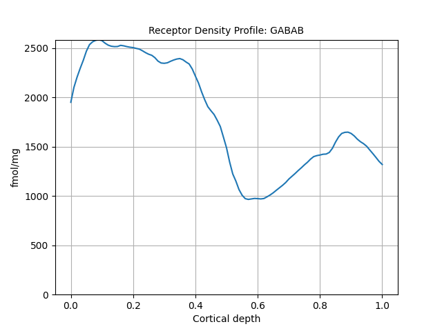
<Axes: title={'center': 'Receptor Density Profile: GABAB'}, xlabel='Cortical depth', ylabel='fmol/mg'>