Cortical cell body distributions

Another regional data feature are cortical distributions of cell bodies. The distributions are measured crom cortical image patches that have been extracted from the original cell-body stained histological sections of the Bigbrain (Amunts et al., 2013), scanned at 1 micrometer resolution. These patches come together with manual annotations of cortical layers. The cell segmentations have been performed using the recently proposed Contour Proposal Networks (CPN; E. Upschulte et al.; https://arxiv.org/abs/2104.03393; https://github.com/FZJ-INM1-BDA/celldetection).

import siibra
import matplotlib.pyplot as plt
from nilearn import plotting

Find cell density profiles for V1. Cortical profile features are combined together as elements to form Compound features. Therefore, we can select the first and only item in the results.

v1 = siibra.get_region("julich 2.9", "v1")
cf = siibra.features.get(v1, siibra.features.cellular.CellDensityProfile)[0]
print(cf.name)

10 Cell Density Profile features

We can browse through the elements with integer index. To illustrate, let us look at the default visualization the first of them, this time using plotly backend. This will actually fetch the cell segmentation data.

print(cf[0].name)
cf[0].plot(backend="plotly")

Cell Density Profile: (13.238324165344238, -65.80000305175781, 8.006086349487305)

The segmented cells are stored in each feature as a numpy array with named columns.

cells = cf[0].cells
print("Number of segmented cells:", len(cells))
cells.head()

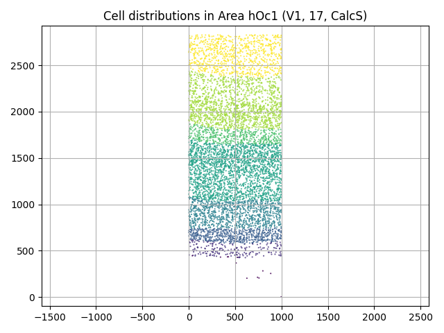
Number of segmented cells: 6298

	x	y	area(micron**2)	layer	label
0	816.108696	1894.260870	138.0	6	103
1	907.913043	1957.173913	92.0	6	126
2	868.972973	1338.702703	37.0	4	132
3	106.000000	1034.674419	43.0	3	173
4	978.034483	994.793103	29.0	3	182

We can, for example, plot the 2D distribution of the cell locations colored by layers:

plt.scatter(cells.x, cells.y, c=cells.layer, s=0.2)
plt.title(f"Cell distributions in {v1.name}")
plt.grid(True)
plt.axis("equal")
plt.tight_layout()

Having the data in data frame format allows further flexibility such as:

layer1_cells = cells.query('layer == 1')
plt.scatter(
    layer1_cells.x, layer1_cells.y,
    s=layer1_cells["area(micron**2)"], c=layer1_cells.label
)
area_layer1 = layer1_cells["area(micron**2)"]
plt.title(f"Mean cell area in layer 1: {area_layer1.mean()}")

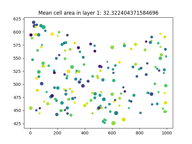
Text(0.5, 1.0, 'Mean cell area in layer 1: 32.322404371584696')

The features also have location information. We can plot their location in BigBrain space:

location = cf[0].anchor.location
print(location)

# fetch the template of the location's space
template = location.space.get_template().fetch()
view = plotting.plot_anat(anat_img=template, cut_coords=tuple(location))
view.add_markers([tuple(location)])

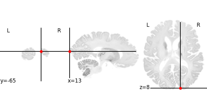
Point in BigBrain microscopic template (histology) [13.238324165344238,-65.80000305175781,8.006086349487305]
/opt/hostedtoolcache/Python/3.8.18/x64/lib/python3.8/site-packages/nilearn/plotting/img_plotting.py:555: RuntimeWarning:

overflow encountered in scalar add

/opt/hostedtoolcache/Python/3.8.18/x64/lib/python3.8/site-packages/nilearn/plotting/img_plotting.py:565: RuntimeWarning:

overflow encountered in scalar add

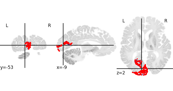
Now let us look into BigBrain intenstiy profiles for V1 left and dispaly the gray matter mesh coordinates on the region mask.

v1left = siibra.get_region("julich 2.9", "v1 left")
cf = siibra.features.get(v1left, "BigBrainIntensityProfile")[0]

mask = v1left.get_regional_map("bigbrain").fetch()  # to highlight the region mask
view2 = plotting.plot_roi(mask, bg_img=template)
view2.add_markers(cf.anchor.location.coordinates, marker_size=5)

Then, for comparison we can plot the profiles %%

cf[0].plot(backend="plotly")