Note
Go to the end to download the full example code.
Access BigBrain high-resolution data
siibra provides access to high-resolution image data parcellation maps defined for the 20 micrometer BigBrain space. The BigBrain is very different from other templates. Its native resolution is 20 micrometer, resulting in about one Terabyte of image data. Yet, fetching the template works the same way as for the MNI templates, with the difference that we can specify a reduced resolution or volume of interest to fetch a feasible amount of image data, or a volume of interest.
We start by selecting an atlas.
import siibra
from nilearn import plotting
Per default, siibra will fetch the whole brain volume at a reasonably reduced resolution.
space = siibra.spaces['bigbrain']
bigbrain_template = space.get_template()
bigbrain_whole_img = bigbrain_template.fetch(resolution_mm=1)
plotting.view_img(bigbrain_whole_img, bg_img=None, cmap='gray')
To see the full resolution, we may specify a bounding box in the physical space. You will learn more about spatial primitives like points and bounding boxes in Locations in reference spaces. For now, we just define a volume of interest from two corner points in the histological space. We specify the points with a string representation, which could be conveniently copy pasted from the interactive viewer siibra explorer. Note that the coordinates can be specified by 3-tuples, and in other ways.
voi = siibra.locations.BoundingBox(
point1="-30.590mm, 3.270mm, 47.814mm",
point2="-26.557mm, 6.277mm, 50.631mm",
space=space
)
bigbrain_chunk = bigbrain_template.fetch(voi=voi)
plotting.view_img(bigbrain_chunk, bg_img=None, cmap='gray')
/actions-runner/_work/siibra-python/siibra-python/examples/02_maps_and_templates/004_access_bigbrain.py:57: UserWarning: Threshold given was 1e-06, but the data has no values below 2.0.
plotting.view_img(bigbrain_chunk, bg_img=None, cmap='gray')
Note that since both fetched image volumes are spatial images with a properly defined transformation between their voxel and physical spaces, we can directly plot them correctly superimposed on each other:
plotting.view_img(
bigbrain_chunk,
bg_img=bigbrain_whole_img,
cmap='magma',
cut_coords=tuple(voi.center)
)
/actions-runner/_work/siibra-python/siibra-python/examples/02_maps_and_templates/004_access_bigbrain.py:63: UserWarning: Threshold given was 1e-06, but the data has no values below 2.0.
plotting.view_img(
/actions-runner/_work/siibra-python/siibra-python/.ci-docs-29154883747-2-notebooks/venv/lib/python3.11/site-packages/numpy/_core/fromnumeric.py:840: UserWarning: Warning: 'partition' will ignore the 'mask' of the MaskedArray.
a.partition(kth, axis=axis, kind=kind, order=order)
/actions-runner/_work/siibra-python/siibra-python/.ci-docs-29154883747-2-notebooks/venv/lib/python3.11/site-packages/nilearn/plotting/image/utils.py:152: RuntimeWarning: overflow encountered in scalar add
black_bg = not (background > 0.5 * (vmin + vmax))
/actions-runner/_work/siibra-python/siibra-python/.ci-docs-29154883747-2-notebooks/venv/lib/python3.11/site-packages/nilearn/plotting/image/utils.py:159: RuntimeWarning: overflow encountered in scalar add
vmean = 0.5 * (vmin + vmax)
Next we select a parcellation which provides a map for BigBrain, and extract labels for the same volume of interest. We choose the cortical layer maps by Wagstyl et al<https://journals.plos.org/plosbiology/article?id=10.1371/journal.pbio.3000678>. Note that siibra will fetch the highest possible resolution if not specified limited by the download size which can be updated with max_bytes
<nibabel.nifti1.Nifti1Image object at 0x7ff8ed8e5b90>
Since we operate in physical coordinates, we can plot both image chunks superimposed, even if their resolution is not exactly identical.
plotting.view_img(mask, bg_img=bigbrain_chunk, opacity=.2, symmetric_cmap=False)
/actions-runner/_work/siibra-python/siibra-python/.ci-docs-29154883747-2-notebooks/venv/lib/python3.11/site-packages/numpy/_core/fromnumeric.py:840: UserWarning: Warning: 'partition' will ignore the 'mask' of the MaskedArray.
a.partition(kth, axis=axis, kind=kind, order=order)
/actions-runner/_work/siibra-python/siibra-python/.ci-docs-29154883747-2-notebooks/venv/lib/python3.11/site-packages/nilearn/plotting/image/utils.py:152: RuntimeWarning: overflow encountered in scalar add
black_bg = not (background > 0.5 * (vmin + vmax))
/actions-runner/_work/siibra-python/siibra-python/.ci-docs-29154883747-2-notebooks/venv/lib/python3.11/site-packages/nilearn/plotting/image/utils.py:159: RuntimeWarning: overflow encountered in scalar add
vmean = 0.5 * (vmin + vmax)
siibra can help us to assign a brain region to the position of the volume of interest. This is covered in more detail in Anatomical assignment. For now, just note that siibra can employ spatial objects from different template spaces. Here it automatically warps the centroid of the volume of interest to MNI space for location assignment.
julich_pmaps = siibra.get_map(space='mni152', parcellation='julich', maptype='statistical')
assignments = julich_pmaps.assign(voi.center)
assignments
1 micron scans of BigBrain sections across the brain can be found as VolumeOfInterest features. The result is a high-resolution image structure, just like the bigbrain template.
hoc5l = siibra.get_region('julich 2.9', 'hoc5 left')
features = siibra.features.get(
hoc5l,
siibra.features.cellular.CellbodyStainedSection
)
# let's see the names of the found features
for f in features:
print(f.name)
#1255: selected 1 micron scans of BigBrain histological sections (v1.0) (cell body staining)
#1307: selected 1 micron scans of BigBrain histological sections (v1.0) (cell body staining)
#1345: selected 1 micron scans of BigBrain histological sections (v1.0) (cell body staining)
#1402: selected 1 micron scans of BigBrain histological sections (v1.0) (cell body staining)
#1454: selected 1 micron scans of BigBrain histological sections (v1.0) (cell body staining)
#1499: selected 1 micron scans of BigBrain histological sections (v1.0) (cell body staining)
#1561: selected 1 micron scans of BigBrain histological sections (v1.0) (cell body staining)
#1600: selected 1 micron scans of BigBrain histological sections (v1.0) (cell body staining)
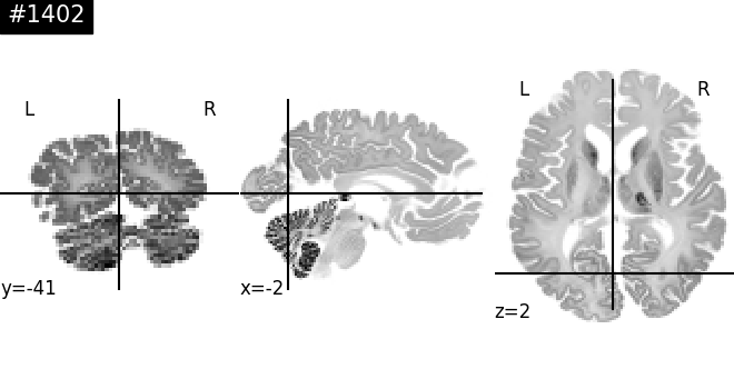
Now fetch the 1 micron section at a lower resolution, and display in 3D space.
section1402 = features[3]
plotting.plot_img(
section1402.fetch(resolution_mm=1),
bg_img=bigbrain_whole_img,
title="#1402",
cmap='gray',
colorbar=False,
)
/actions-runner/_work/siibra-python/siibra-python/examples/02_maps_and_templates/004_access_bigbrain.py:110: UserWarning: Could not determine cut coords: All voxels were masked by the thresholding. Returning the center of mass instead.
plotting.plot_img(
<nilearn.plotting.displays._slicers.OrthoSlicer object at 0x7ff8f1547a50>
Let’s fetch a crop inside hoc5 at full resolution. We intersect the bounding box of hoc5l and the section.
hoc5_bbox = hoc5l.get_boundingbox('bigbrain').intersection(section1402)
print(f"Size of the bounding box: {hoc5_bbox.shape}")
# this is quite large, so we shrink it
voi = hoc5_bbox.zoom(0.1)
crop = section1402.fetch(voi=voi)
plotting.plot_img(crop, bg_img=None, cmap="gray", display_mode="y", colorbar=False)
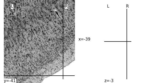
Size of the bounding box: (13.716000000000001, 0.020000000000003126, 16.129)
/actions-runner/_work/siibra-python/siibra-python/examples/02_maps_and_templates/004_access_bigbrain.py:127: UserWarning: Too many cuts requested for the data: n_cuts=7, data size=1.
plotting.plot_img(crop, bg_img=None, cmap="gray", display_mode="y", colorbar=False)
<nilearn.plotting.displays._slicers.YSlicer object at 0x7ff868db26d0>
Total running time of the script: (1 minutes 37.846 seconds)
Estimated memory usage: 890 MB