
Note
Go to the end to download the full example code.
High-resolution Rat Local Field Potential Atlas
Local field potentials (LFPs) capture electrophysiological activity recorded from neural tissue. In this example, we query LFP recordings and spectra from a high-resolution rat atlas dataset linked to regions of the Waxholm Space atlas.
import siibra
We start by selecting the Waxholm Space parcellation and choosing the caudate putamen as the anatomical region of interest.
waxholm = siibra.parcellations.get("waxholm v4")
ventral_orbital = waxholm.get_region("Ventral orbital area")
Query all local field potential features linked to the caudate putamen.
lfp_ventral_orbital = siibra.features.get(
    ventral_orbital,
    siibra.features.functional.LocalFieldPotential
)
print(f"Found {len(lfp_ventral_orbital)} local field potentials")
Found 507 local field potentials
LFP features provide metadata fields that can be used to filter the results. The options can be accessed from siibra.vocabularies:
siibra.vocabularies.get_lfp_options()
{'pathology': {'none', 'intact hemisphere in 6-OHDA hemilesioned animal', 'lesioned hemisphere in 6-OHDA hemilesioned animal'}, 'pharmacology': {'skf82958', 'lsd', 'amphetamine', 'sumanirole', 'doi', 'baseline', 'levodopa', 'mk801', 'ketamine', 'pcp'}, 'signal_quality': {'atypical', 'typical', 'strongly atypical'}}
Here, we restrict the query to baseline recordings with typical signal quality.
specs = {
    "pharmacology": "baseline",
    "signal_quality": "typical",
    "pathology": "lesioned hemisphere in 6-OHDA hemilesioned animal",
}
fts_w_specs = siibra.features.get(
    ventral_orbital,
    siibra.features.functional.LocalFieldPotential,
    **specs
)
print(f"Found {len(fts_w_specs)} local field potentials with specs: {specs}")
Found 101 local field potentials with specs: {'pharmacology': 'baseline', 'signal_quality': 'typical', 'pathology': 'lesioned hemisphere in 6-OHDA hemilesioned animal'}
The same metadata options can also be used to search for atypical recordings. This allows comparing different subsets of the available electrophysiological data.
specs["signal_quality"] = "atypical"
fts_w_specs = siibra.features.get(
    ventral_orbital,
    siibra.features.functional.LocalFieldPotential,
    **specs
)
print(f"Found {len(fts_w_specs)} local field potentials with specs: {specs}")
Found 5 local field potentials with specs: {'pharmacology': 'baseline', 'signal_quality': 'atypical', 'pathology': 'lesioned hemisphere in 6-OHDA hemilesioned animal'}
Inspect the metadata of one LFP feature. These fields describe the subject, recording session, pharmacological condition, pathology, and signal quality.
f = lfp_ventral_orbital[0]
print("subject:", f.subject)
print("session:", f.session)
print("pharmacology:", f.pharmacology)
print("pathology:", f.pathology)
print("signal_quality:", f.signal_quality)
subject: sub-02
session: ses-01
pharmacology: levodopa
pathology: intact hemisphere in 6-OHDA hemilesioned animal
signal_quality: typical
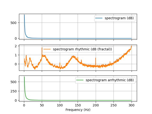
We can plot spectra using any regions including the whole Waxholm parcellation using plot_spectra` method. Here selecting Ventral orbital area, typical recordings from the healthy animals with no pharmacological treatment.
specs = dict(
    pathology="none",
    pharmacology="baseline",
    signal_quality="typical",
)
lfp_spectrum_w_specs = siibra.features.get(
    ventral_orbital,
    siibra.features.functional.LocalFieldPotential,
    **specs
)
siibra.features.functional.LocalFieldPotential.plot_spectra(lfp_spectrum_w_specs)
Alternatively, region-wise potentials can be queried already grouped for ease of navigation. These are divided by pathology, pharmacology, and signal quality tuples.
lfp_spectrum_ventral_orbital = siibra.features.get(
    ventral_orbital,
    siibra.features.functional.RegionalLocalFieldPotential,
    **specs
)
lfp_spectrum_ventral_orbital[0].data
Plotting functionality requires no further input
lfp_spectrum_ventral_orbital[0].plot(backend='plotly')
Total running time of the script: (0 minutes 38.989 seconds)
Estimated memory usage: 123 MB